MILP Solve Time vs. Feature & Sample Dimensions

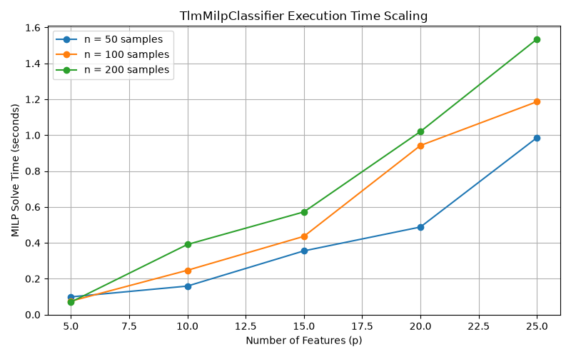
This example evaluates how execution time scales with feature count \(p\) and sample size \(n\) when optimizing exact ternary weights via MILP.

import time
import matplotlib.pyplot as plt
from sklearn.datasets import make_classification
from tlmnet import TlmMilpClassifier

feature_counts = [5, 10, 15, 20, 25]
sample_sizes = [50, 100, 200]
results: dict[int, list[float]] = {n: [] for n in sample_sizes}

for n in sample_sizes:
    for p in feature_counts:
        X, y = make_classification(
            n_samples=n, n_features=p, n_informative=min(p, 3), random_state=42
        )
        clf = TlmMilpClassifier(max_features=5, C=1.0)

        start = time.time()
        clf.fit(X, y)
        elapsed = time.time() - start

        results[n].append(elapsed)

plt.figure(figsize=(8, 5))
for n in sample_sizes:
    plt.plot(feature_counts, results[n], marker="o", label=f"n = {n} samples")

plt.xlabel("Number of Features (p)")
plt.ylabel("MILP Solve Time (seconds)")
plt.title("TlmMilpClassifier Execution Time Scaling")
plt.legend()
plt.grid(True)
plt.tight_layout()
plt.show()