Multilabel Text Document Classification with CALF One-vs-Rest

This example demonstrates how Calf performs multi-class text classification using a One-vs-Rest strategy (OneVsRestClassifier).

While Calf is natively a binary estimator, wrapping it in OneVsRestClassifier allows it to evaluate multi-class document categories (such as the 20 Newsgroups dataset). We compare execution time, model sparsity, and accuracy against standard Scikit-Learn classifiers including Ridge, Perceptron, LinearSVC, Naive Bayes, and Random Forest.

Imports and Dataset Loading

from time import time
import matplotlib.pyplot as plt
import numpy as np

from sklearn.datasets import fetch_20newsgroups
from sklearn.ensemble import RandomForestClassifier
from sklearn.feature_extraction.text import TfidfVectorizer
from sklearn.linear_model import (
    Perceptron,
    RidgeClassifier,
    SGDClassifier,
)
from sklearn.metrics import accuracy_score
from sklearn.multiclass import OneVsRestClassifier
from sklearn.naive_bayes import MultinomialNB
from sklearn.neighbors import KNeighborsClassifier
from sklearn.svm import LinearSVC

from calfcv import Calf

# Select 4 categories for benchmarking
categories = [
    "alt.atheism",
    "talk.religion.misc",
    "comp.graphics",
    "sci.space",
]

print("Loading 20 newsgroups dataset (cached locally)...")
data_train = fetch_20newsgroups(
    subset="train", categories=categories, shuffle=True, random_state=42
)
data_test = fetch_20newsgroups(
    subset="test", categories=categories, shuffle=True, random_state=42
)

# Extract TF-IDF sparse features
vectorizer = TfidfVectorizer(sublinear_tf=True, max_df=0.5, stop_words="english")
X_train = vectorizer.fit_transform(data_train.data)
X_test = vectorizer.transform(data_test.data)

y_train, y_test = data_train.target, data_test.target

print(f"Train Samples: {X_train.shape[0]}, Features: {X_train.shape[1]}")
print(f"Test Samples:  {X_test.shape[0]}, Features: {X_test.shape[1]}")

Loading 20 newsgroups dataset (cached locally)...
Train Samples: 2034, Features: 33809
Test Samples:  1353, Features: 33809

Benchmark Function

def benchmark(clf, name):
    print("=" * 80)
    print(f"Training: {name}")

    t0 = time()
    clf.fit(X_train, y_train)
    train_time = time() - t0

    t0 = time()
    pred = clf.predict(X_test)
    test_time = time() - t0

    score = accuracy_score(y_test, pred)
    print(
        f"Train Time: {train_time:.3f}s | Test Time: {test_time:.3f}s | Accuracy: {score:.3f}"
    )

    return name, score, train_time, test_time

Evaluate Classifiers

results = []

# CALF One-vs-Rest
results.append(
    benchmark(OneVsRestClassifier(Calf(order_col=True, verbose=False)), "Calf OVR")
)

# Standard Baselines
results.append(benchmark(RidgeClassifier(tol=1e-2, solver="lsqr"), "Ridge"))
results.append(benchmark(Perceptron(), "Perceptron"))
# Using SGD configuration to replace deprecated PassiveAggressiveClassifier
results.append(
    benchmark(
        SGDClassifier(loss="hinge", penalty=None, learning_rate="pa1", eta0=1.0),
        "Passive-Aggressive",
    )
)
results.append(benchmark(KNeighborsClassifier(n_neighbors=10), "kNN"))
results.append(benchmark(RandomForestClassifier(n_estimators=100), "Random Forest"))
results.append(benchmark(LinearSVC(penalty="l2", dual=False, tol=1e-3), "L2 LinearSVC"))
results.append(benchmark(SGDClassifier(penalty="l1"), "L1 SGD"))
results.append(benchmark(MultinomialNB(alpha=0.01), "Multinomial NB"))

================================================================================
Training: Calf OVR
Train Time: 69.771s | Test Time: 0.011s | Accuracy: 0.823
================================================================================
Training: Ridge
Train Time: 0.082s | Test Time: 0.003s | Accuracy: 0.899
================================================================================
Training: Perceptron
Train Time: 0.118s | Test Time: 0.002s | Accuracy: 0.888
================================================================================
Training: Passive-Aggressive
Train Time: 0.048s | Test Time: 0.002s | Accuracy: 0.902
================================================================================
Training: kNN
Train Time: 0.002s | Test Time: 0.099s | Accuracy: 0.858
================================================================================
Training: Random Forest
Train Time: 2.644s | Test Time: 0.116s | Accuracy: 0.842
================================================================================
Training: L2 LinearSVC
Train Time: 0.169s | Test Time: 0.002s | Accuracy: 0.900
================================================================================
Training: L1 SGD
Train Time: 0.189s | Test Time: 0.003s | Accuracy: 0.890
================================================================================
Training: Multinomial NB
Train Time: 0.008s | Test Time: 0.002s | Accuracy: 0.899

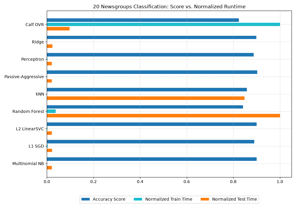
Visualize Performance Comparison

indices = np.arange(len(results))
clf_names, scores, train_times, test_times = zip(*results)

train_times_norm = np.array(train_times) / np.max(train_times)
test_times_norm = np.array(test_times) / np.max(test_times)

fig, ax = plt.subplots(figsize=(10, 7))
ax.set_title("20 Newsgroups Classification: Score vs. Normalized Runtime")

ax.barh(indices, scores, 0.2, label="Accuracy Score", color="#1f77b4")
ax.barh(
    indices + 0.25,
    train_times_norm,
    0.2,
    label="Normalized Train Time",
    color="#17becf",
)
ax.barh(
    indices + 0.5, test_times_norm, 0.2, label="Normalized Test Time", color="#ff7f0e"
)

ax.set_yticks(indices + 0.25)
ax.set_yticklabels(clf_names)
ax.invert_yaxis()  # Put Calf OVR at the top of the chart

# Place legend outside the plot area below the chart
ax.legend(loc="upper center", bbox_to_anchor=(0.5, -0.1), ncol=3)
ax.grid(True, linestyle="--", alpha=0.5)

plt.tight_layout()
plt.show()