Feature Selection Sparsity: CALF vs. L1 & RFE

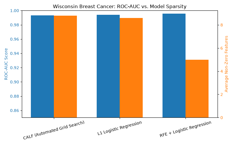
This example compares the coarse feature selection of CalfCV against L1-penalized Logistic Regression (Lasso) and Recursive Feature Elimination (RFE) on the Wisconsin Breast Cancer dataset.

While continuous models often assign fractional weights across many correlated features, CalfCV performs discrete forward selection using coarse integer weights (+1, -1). This produces highly sparse, interpretable models with competitive ROC-AUC performance.

CalfCV automatically optimizes CALF’s weight search grid, AUC tolerance, and column pre-sorting strategy via internal cross-validation.

Imports and Dataset Loading

import matplotlib.pyplot as plt
import numpy as np
import pandas as pd
from sklearn.datasets import load_breast_cancer
from sklearn.feature_selection import RFE
from sklearn.linear_model import LogisticRegression
from sklearn.metrics import roc_auc_score
from sklearn.model_selection import StratifiedKFold, cross_validate
from sklearn.pipeline import make_pipeline
from sklearn.preprocessing import StandardScaler

from calfcv import CalfCV

X, y = load_breast_cancer(return_X_y=True, as_frame=True)

cv = StratifiedKFold(n_splits=5, shuffle=True, random_state=42)

Define Comparison Estimators and Pipelines Note: CalfCV automatically prepends StandardScaler internally when X is dense, so wrapping it with an external StandardScaler is redundant.

pipelines = {
    "CALF (Automated Grid Search)": CalfCV(
        grid=[(-1, 1), (-1, 0, 1)],
        auc_tol=[0.001, 0.005, 0.01],
        order_col=[True, False],
        cv=5,
        n_jobs=-1,
    ),
    "L1 Logistic Regression": make_pipeline(
        StandardScaler(),
        LogisticRegression(l1_ratio=1, solver="liblinear", C=0.1, random_state=42),
    ),
    "RFE + Logistic Regression": make_pipeline(
        StandardScaler(),
        RFE(
            estimator=LogisticRegression(l1_ratio=0, solver="liblinear"),
            n_features_to_select=5,
        ),
    ),
}

Evaluate Models via Cross-Validation

results = []

for name, pipe in pipelines.items():
    cv_res = cross_validate(pipe, X, y, cv=cv, scoring="roc_auc", return_estimator=True)

    nonzero_counts = []
    for est in cv_res["estimator"]:
        if "CALF" in name:
            calfcv_model = (
                est.named_steps["calfcv"] if hasattr(est, "named_steps") else est
            )
            nonzero_counts.append(np.count_nonzero(calfcv_model.best_coef_))
        elif "rfe" in getattr(est, "named_steps", {}):
            nonzero_counts.append(np.sum(est.named_steps["rfe"].support_))
        else:
            coefs = est.named_steps["logisticregression"].coef_
            nonzero_counts.append(np.count_nonzero(coefs))

    results.append(
        {
            "Model": name,
            "Mean ROC-AUC": np.mean(cv_res["test_score"]),
            "Std ROC-AUC": np.std(cv_res["test_score"]),
            "Avg Active Features": np.mean(nonzero_counts),
        }
    )

df_results = pd.DataFrame(results)

Visualize ROC-AUC vs. Sparsity

fig, ax1 = plt.subplots(figsize=(8, 5))

x = np.arange(len(df_results))
width = 0.35

rects1 = ax1.bar(
    x - width / 2,
    df_results["Mean ROC-AUC"],
    width,
    label="Mean ROC-AUC",
    color="#1f77b4",
)
ax1.set_ylabel("ROC-AUC Score", color="#1f77b4")
ax1.set_ylim(0.85, 1.0)
ax1.tick_params(axis="y", labelcolor="#1f77b4")

ax2 = ax1.twinx()
rects2 = ax2.bar(
    x + width / 2,
    df_results["Avg Active Features"],
    width,
    label="Active Features",
    color="#ff7f0e",
)
ax2.set_ylabel("Average Non-Zero Features", color="#ff7f0e")
ax2.tick_params(axis="y", labelcolor="#ff7f0e")

ax1.set_xticks(x)
ax1.set_xticklabels(df_results["Model"], rotation=15)
ax1.set_title("Wisconsin Breast Cancer: ROC-AUC vs. Model Sparsity")

fig.tight_layout()
plt.show()

Detailed Model Inspection (Single Fit on Full Data)

print("\n" + "=" * 50)
print("DETAILED MODEL INSPECTION (Full Dataset Fit)")
print("=" * 50)

for name, pipe in pipelines.items():
    # Fit model/pipeline on the entire dataset
    pipe.fit(X, y)

    # Calculate Full-Data AUC
    if hasattr(pipe, "predict_proba"):
        y_score = pipe.predict_proba(X)[:, 1]
    else:
        y_score = pipe.decision_function(X)

    auc = roc_auc_score(y, y_score)

    print(f"\n--- {name} ---")
    print(f"Full-Data ROC-AUC: {auc:.4f}")

    # Extract weights based on the specific estimator API
    if "CALF" in name:
        model = pipe.named_steps["calfcv"] if hasattr(pipe, "named_steps") else pipe
        print(f"[CalfCV Optimal Hyperparameters Found]: {model.best_params_}")
        weights = np.squeeze(model.best_coef_)
        active_mask = weights != 0
    elif "rfe" in getattr(pipe, "named_steps", {}):
        rfe = pipe.named_steps["rfe"]
        weights = np.zeros(X.shape[1])
        # Map the inner estimator's weights back to the selected support features
        weights[rfe.support_] = np.squeeze(rfe.estimator_.coef_)
        active_mask = rfe.support_
    else:
        model = pipe.named_steps["logisticregression"]
        weights = np.squeeze(model.coef_)
        active_mask = weights != 0

    selected_df = pd.DataFrame(
        {
            "Feature": np.array(X.columns)[active_mask],
            "Weight": np.round(weights[active_mask], 4),
        }
    )

    print(f"Total Selected Features: {active_mask.sum()}")
    print(selected_df.to_string(index=False))

==================================================
DETAILED MODEL INSPECTION (Full Dataset Fit)
==================================================

--- CALF (Automated Grid Search) ---
Full-Data ROC-AUC: 0.9910
[CalfCV Optimal Hyperparameters Found]: {'classifier__auc_tol': 0.005, 'classifier__grid': (-1, 1), 'classifier__order_col': False, 'classifier__verbose': False}
Total Selected Features: 6
        Feature  Weight
    mean radius      -1
 mean perimeter      -1
mean smoothness      -1
 mean concavity      -1
   worst radius      -1
  worst texture      -1

--- L1 Logistic Regression ---
Full-Data ROC-AUC: 0.9956
Total Selected Features: 8
             Feature  Weight
 mean concave points -0.6291
        radius error -0.5153
        worst radius -2.3459
       worst texture -0.6947
    worst smoothness -0.2570
     worst concavity -0.0634
worst concave points -0.8126
      worst symmetry -0.1949

--- RFE + Logistic Regression ---
Full-Data ROC-AUC: 0.9961
Total Selected Features: 5
             Feature  Weight
        radius error -1.5515
        worst radius -1.9615
       worst texture -1.3908
          worst area -1.9081
worst concave points -2.7258

Interpretation: Clinical Transparency via Coarse Weighting

The output above illustrates the fundamental trade-off between continuous mathematical optimization and clinical interpretability.

• L1 & RFE (Continuous Weights): These estimators achieve high AUCs using complex, fractional coefficients (e.g., -2.3459). They aggressively prune redundant features but force the practitioner to rely on a fractional black box.

• CALF (Integer Weights): CALF restricts weights to strictly -1 or +1. Instead of assigning a massive fractional penalty to a single dominant feature, it builds magnitude by stacking -1 weights across multiple correlated indicators (e.g., mean radius, mean perimeter, mean area).

How the Threshold Works: Because the data is scaled to have a mean of 0, the -1 weights act as penalties for values above the population average. If a patient’s tumor is larger or more irregular than average, those positive standard deviations are multiplied by -1, driving the composite sum downward. The features pool together into a single aggregate score. To predict the benign class, the final integer-weighted sum must simply be greater than or equal to zero.