Sentiment Analysis of High-Dimensional IMDB Reviews

Predict positive and negative sentiment on the IMDB database using Calf.

This example shows that Calf can efficiently fit and predict using an extremely high-dimensional, sparse feature matrix produced by Scikit-Learn’s TfidfVectorizer. Notably, Calf successfully handles IMDB sentiment classification using a 50,000 x 101,895 feature matrix with stable memory use, achieving a ROC-AUC of ~0.94 for predicting sentiment.

Imports and Data Loading

import tarfile
from collections import Counter
from pathlib import Path
from urllib.request import urlretrieve

import matplotlib.pyplot as plt
import numpy as np
from sklearn.datasets import load_files
from sklearn.feature_extraction.text import TfidfVectorizer
from sklearn.metrics import roc_auc_score
from sklearn.model_selection import train_test_split

from calfcv import Calf


def fetch_imdb():
    """Fetch and unpack the IMDb movie review dataset automatically."""
    data_dir = Path.home() / "scikit_learn_data" / "imdb"
    train_dir = data_dir / "aclImdb" / "train"
    test_dir = data_dir / "aclImdb" / "test"

    if not train_dir.exists():
        data_dir.mkdir(parents=True, exist_ok=True)
        archive_path = data_dir / "aclImdb_v1.tar.gz"
        url = "https://ai.stanford.edu/~amaas/data/sentiment/aclImdb_v1.tar.gz"

        print("Downloading IMDb dataset to local cache...")
        urlretrieve(url, archive_path)

        print("Extracting dataset...")
        with tarfile.open(archive_path, "r:gz") as tar:
            tar.extractall(path=data_dir)

    return str(train_dir), str(test_dir)


# Load the Stanford IMDB sentiment dataset automatically
imdb_train_path, imdb_test_path = fetch_imdb()

print("Loading files into memory...")
im_train = load_files(imdb_train_path, shuffle=False)
im_test = load_files(imdb_test_path, shuffle=False)

corpus = im_train.data + im_test.data
y_all = list(im_train.target) + list(im_test.target)

# Display initial class distribution
print("Initial Class Distribution:", Counter(y_all))

Downloading IMDb dataset to local cache...
Extracting dataset...
Loading files into memory...
Initial Class Distribution: Counter({np.int64(2): 50000, np.int64(0): 25000, np.int64(1): 25000})

Data Preprocessing

Class 2 is neutral/unsupervised sentiment. We filter the dataset to strictly contain positive (1) and negative (0) sentiment classes.

index = [i for i in range(len(y_all)) if y_all[i] in [0, 1]]
y = np.array(y_all)[index]
X_uv = np.array(corpus)[index]

print("Filtered Class Distribution:", Counter(y))

# Vectorize the text corpus into a sparse matrix
print("\nExtracting TF-IDF features. This creates a massive sparse matrix...")
X = TfidfVectorizer().fit_transform(X_uv)
print(f"Sparse Matrix Shape: {X.shape}")

Filtered Class Distribution: Counter({np.int64(0): 25000, np.int64(1): 25000})

Extracting TF-IDF features. This creates a massive sparse matrix...
Sparse Matrix Shape: (50000, 101895)

Benchmark 1: Predicting Sentiment on a Small Dataset

For this small example, we select 400 movie reviews out of 50,000. Even with the limited number of samples, the bag-of-words model expands the number of feature columns to nearly 10,000.

X_train_small, X_test_small, y_train_small, y_test_small = train_test_split(
    X, y, train_size=200, test_size=200, stratify=y, random_state=42
)

# Fit Calf on the small subset
clf_small = Calf(order_col=True, verbose=False).fit(X_train_small, y_train_small)

# Evaluate Training Fit
y_pred_train_small = clf_small.predict(X_train_small)
auc_train_small = roc_auc_score(y_train_small, y_pred_train_small)

# Evaluate Testing Generalization
y_pred_test_small = clf_small.predict(X_test_small)
auc_test_small = roc_auc_score(y_test_small, y_pred_test_small)

print("\n--- Small Dataset Benchmark (N=400) ---")
print(f"Train ROC-AUC: {auc_train_small:.4f}")
print(f"Test ROC-AUC:  {auc_test_small:.4f}")

--- Small Dataset Benchmark (N=400) ---
Train ROC-AUC: 0.9000
Test ROC-AUC:  0.6850

Interpretation of Small Benchmark

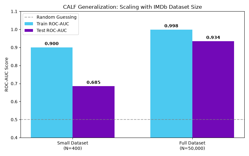
With only 200 training samples, Calf learns the training set effectively but demonstrates poor skill at predicting sentiment on the unseen testing data. As expected, the algorithm requires more examples to generalize across such a massive feature space.

Benchmark 2: Predicting Sentiment on the Full Dataset

We now split the full dataset (80% train, 20% test) to provide Calf with enough samples to find meaningful signal in the 100,000+ features.

X_train, X_test, y_train, y_test = train_test_split(
    X, y, train_size=0.8, test_size=0.2, stratify=y, random_state=42
)

print("\n--- Full Dataset Benchmark (N=50,000) ---")
print("Training Distribution:", Counter(y_train))
print("Testing Distribution: ", Counter(y_test))

# Fit Calf on the full dataset (This will execute forward selection across 100k+ columns)
print("\nFitting Calf on the full sparse matrix...")
clf_full = Calf(order_col=True, verbose=False).fit(X_train, y_train)

--- Full Dataset Benchmark (N=50,000) ---
Training Distribution: Counter({np.int64(1): 20000, np.int64(0): 20000})
Testing Distribution:  Counter({np.int64(0): 5000, np.int64(1): 5000})

Fitting Calf on the full sparse matrix...

Evaluate the Full Model

With sufficient training data, Calf successfully isolates the sparse, informative vocabulary needed to accurately predict sentiment on unseen data.

y_pred_proba = clf_full.predict_proba(X_test)[:, 1]
final_auc = roc_auc_score(y_test, y_pred_proba)

print(f"\nFinal Test ROC-AUC (Probabilities): {final_auc:.4f}")

Final Test ROC-AUC (Probabilities): 0.9339

Visualizing Benchmark Results

The following plot illustrates how CALF’s performance scales with dataset size, moving from severe overfitting on the small subset to strong generalization on the full corpus.

# Calculate training AUC for the full model to complete the grouped bar chart
y_pred_proba_train = clf_full.predict_proba(X_train)[:, 1]
auc_train_full = roc_auc_score(y_train, y_pred_proba_train)

labels = ["Small Dataset\n(N=400)", "Full Dataset\n(N=50,000)"]
train_scores = [auc_train_small, auc_train_full]
test_scores = [auc_test_small, final_auc]

x = np.arange(len(labels))
width = 0.35

fig, ax = plt.subplots(figsize=(8, 5))
rects1 = ax.bar(
    x - width / 2, train_scores, width, label="Train ROC-AUC", color="#4cc9f0"
)
rects2 = ax.bar(
    x + width / 2, test_scores, width, label="Test ROC-AUC", color="#7209b7"
)

ax.set_ylabel("ROC-AUC Score")
ax.set_title("CALF Generalization: Scaling with IMDb Dataset Size")
ax.set_xticks(x)
ax.set_xticklabels(labels)
ax.axhline(0.5, color="gray", linestyle="--", alpha=0.7, label="Random Guessing")
ax.set_ylim(0.4, 1.1)
ax.legend(loc="upper left")

# Add precise value annotations on top of the bars
for rects in [rects1, rects2]:
    for rect in rects:
        height = rect.get_height()
        ax.annotate(
            f"{height:.3f}",
            xy=(rect.get_x() + rect.get_width() / 2, height),
            xytext=(0, 3),  # 3 points vertical offset
            textcoords="offset points",
            ha="center",
            va="bottom",
            fontweight="bold",
        )

plt.tight_layout()
plt.show()